It's been more than a year since I last updated my blog, but worry not, I am back! Yeah you heard and read it right, I am back from blogging. Though, it may take some time to write another new article but I will publish and post again from time to time. It was last September since I posted my latest article, (wow it seems ages ago).
Where did i go? After graduation, I reviewed for my ECE board exam last April 2015. And luckily, I passed both the Electronics Engineering and Electronics Technician examinations (a round of applause please :) ). Yes, now I am a licensed engineer and technician, expect to have a more advance projects, tutorials and circuitry to be posted here. But I can still post the projects I made during my college years so that all those electronics enthusiasts can make it as well. I will also posts new technologies I researched, trending gadgets and it's reviews so that you are always updated. You, my followers, are the most important.
So sit back, enjoy and wait for my new posts and technologies. You will be amazed. Your waiting is worth it. So all of my followers out there, visit my blog once again and read it. Thanks guys!
By the way, if you have any projects, circuits or anything under the sun of electronics you want to ask me, or be made by me, you are all free and welcome to ask me. Just like the saying goes, there is no harm in trying or asking, but as long as it is feasible and not toooo much expensive. My budget is tight right now and building and making expensive projects may took a longer time. You can also ask me to do some circuits simulation and the likes. I am using Proteus ISIS for my circuit simulation, to check whether the circuits will work as designed or not, and I am using EagleCAD for my PCB layouting.
I think I will make a tutorial about this programs, hmmmmm now that is an idea. Penny for your thoughts? Thanks again and have fun always!
PS: To all those who had commented (if there are) and took a long time to have a reply, You have my sincerest apologies, I am really busy and hoping you will still have a comment and visit my blog once again.

image form wikipedia.org
Abstract
This post compares the complex instruction set and reduced instruction set computer design philosophies. Typical characteristics, instructions, and advantages and disadvantages of each philosophy are explained. This paper then proceeds to describe how complex instruction set computers (CISC) and reduced instruction set computers (CISC) have been combined to form a hybrid known as a Complex/Reduced instruction set Computer (CRISC).
Introduction
Two basic computer design philosophies predominant in the market today are the complex instruction set and the reduced instruction set. Immediately, one might be lead to believe by their names that the size of the instruction sets is what distinguishes the two, but the differences extend much further. These philosophies differ in their instruction lengths, addressing modes, number of registers, and the number of clock cycles needed to execute an instruction.
1. CISC
Complex instructions came about in order to maximize the performance of early computers. At that time, computers executed instructions sequentially. The first instruction had to complete the execution cycle before the next instruction could begin. Designers combined sequences of instructions into single instructions. This reduced the amount of time spent retrieving instructions from memory, although these instructions did require multiple clocks cycles to execute.
1.1 Characteristics of CISC
CISC philosophy used microcode to simplify the computer's architecture. In a micro programmed system, the ROM contains a group of microcode instructions that correspond with each machine-language instruction. When a machine-language instruction arrives at the processor, it executes the corresponding series of microcode instructions. In a nutshell, microcode acts as a transition layer between the instructions and the electronics of the computer. This also improved performance, since instructions could be retrieved up to ten times faster from ROM than from main memory. Other advantages of using microcode included fewer transistors, easier implementation of new chips, and a micro programmed design can be easily modified to handle new instruct ions sets.
Another characteristic of complex instructions set is their variable-length instruction format. Variable-length instructions were used to limit the amount of wasted space, although they do require special decoding circuits that count bytes within words and frame the instructions according to their byte length. In the VAX, binary and arithmetic operations have two or three operands, while string operations have three or five operands.
A large number of addressing modes also characterizes complex instruction set computers. The VAX, an example of a complex instruction set computer, has the following modes: to/from a register, to/from a specific location in memory, to/from an address pointed to by a register, to/from an address pointed to by a memory location, to/from an address offset from a base address in a register, to/from an address offset from a base address in memory, etc…. Due to the large number of addressing modes, there are more than 30,000 versions of integer add in the VAX.
Another characteristic of the CISC design philosophy is the small number of general-purpose registers, typically about 8 registers. This is a result of having instructions, which can operate directly on memory.
1.2 Advantages of CISC
Advantages of complex instruction set machines include
- it is less expensive compared to others since it uses a microcode doesn't need to hardwire a control unit
- More compatible because new computers would contain intructions given to the earlier computers
- Fewer instructions are needed to implement a given task, which gives more efficient use of memory
- More instructions can fit into the cache, since the instructions are not a fixed size.
1.3 Disadvantages of CISC
With all these advantages of CISC it still had its drawbacks:
-More complex instruction sets and chip hardware as computers progressesd.
- Since there are more and different instructions, it will take different amount of time to execute.
- Many instructions are not used frequently; Approximately 20% of the available instructions are used in a typical program
1.4 Computers implementing a complex instruction set
The VAX is one example of a CISC. As stated above, it has a large number of addressing modes. Another CISC characteristic it exhibits is variable-length instructions. Binary and arithmetic operations require 2 or 3 operands, but string operations need 3 or 5 operands.
Another computer family that is classified as a complex instruction set computer is the Motorola 68000 family. It contains few general-purpose registers: 8 data registers and 8 address registers. It also uses variable-length instructions. Each inst ruction in one of these computers requires 0, 1, or 2 operands.
Other typical complex instruction set computers include the IBM 370 and Intel's 80x86 line of computers.
2. RISC
In the mid 1970s, developments in technology made RISC attractive to computer designers. Some of these developments were great increases in memory size with corresponding decreases in cost, high-speed caches, advanced compilers, and better pipelining. Due to these developments, IBM designed the first reduced instruction set computer.
2.1 Characteristics of RISC
RISC architecture makes use of a small set of simplified instructions in attempt to improve performance. These instructions consist mostly of register-to-register operations. Only load and store instructions access memory. Sinc e almost all instructions make use of register addressing, there are only a few addressing modes in a reduced instruction set computer and there are a large number of general-purpose registers. For example, a PowerPC has 32 registers.
Another way in which reduced instruction set computers sought to improve performance was to have most instructions complete execution in one machine cycle. Pipelining was a key technique in achieving this. Pipelining allows the next instruction to enter the execution cycle while the previous instruction is still processing.
Another technique utilized by reduced instruction set machines is prefetching coupled with speculative execution. If the processor has fetched a branch instruction, it does not wait to see if the condition has been met. It "guesses" whether or not the condition will be met, and begins execution of the corresponding code. If the processor guessed correctly, it has gained time. If the processor has guessed incorrectly, the results are discarded and there is no loss.
Reduced instruction set machines, unlike complex instruction set machine, use same length instructions so that the instructions are aligned on word boundaries and may be fetched in a single operation. Typically, a reduced instruction set computer stores its instruction in 32 bits.
RISC microprocessors also emphasize floating-point performance making them popular with the scientific community whose applications do more floating-point math. For this reason, most RISC microprocessors have floating-point units (FPUs) built in.
2.2 Advantages of RISC
Advantages of a reduced instruction set machine:
- Faster
- Simpler hardware
- Shorter design cycle due to simpler hardware
- Lower cost since more parts can be placed on a single chip
2.3 Disadvantages of RISC
Drawbacks of a reduced instruction set computer include
- Programmer must pay close attention to instruction scheduling so that the processor does not spend a large amount of time waiting for an instruction to execute
- Debugging can be difficult due to the instruction scheduling
- Require very fast memory systems to feed them instructions
2.4 Computers implementing a reduced instruction set
The PowerPC is a typical reduced instruction set computer. It contains many general-purpose registers (32 in all) and a floating-point unit. It also takes advantage of pipelining to approach the goal of one instruction per clock cycle. Perfecting and speculative execution are other methods the PowerPC uses to speed execution of instructions.
Another processor that implements a RISC architecture is the SPARC. In the SPARC, all instructions are 32-bits in length. Another RISC feature of the SPARC is that only load and store instructions are allowed to access memory. Arithmetic operations are performed only on values in the registers.
Other computers classified as having reduced instruction sets are the MIPS and the Alpha.
3. CRISC
Today, the distinction between RISC and CISC is becoming rather fuzzy. The first hints of RISC technology began to appear in Intel's 80x86 processor in 1989, when the 486 had a FPU, more hard-wired instruction logic, and pipelining. Other manufacturers have followed suit such as Cyrix. Cyrix's M1 also takes advantage of pipelining to increase instruction execution. Another RISC characteristic the M1 has borrowed is a large number of general-purpose registers. The M1 has 32 general-purpose registers by using a technique called dynamic register naming, which makes it appear as if there are only 8 registers in use at a time. This preserves compatibility with existing software that expects to see only 8 registers.
3.1 Computers that implement CRISC
One computer that exhibits features of both CISC and RISC is the Cyrix M1. The M1 has the same micro-architecture as the Intel 80x86 family of complex instruction set machines. It has 32 general-purpose registers as a typical reduced instruction set computers, but by using a technique called dynamic register naming, only 8 registers are visible at a time. This permits the M1 to preserve compatibility with existing software.
One of the examples of another CISC/RISC hybrid is the Pentium. Since, it uses variable-length instructions with few general-purpose registers in order to instruct the computer what it should do, but it also adopts RISC-like features.
Conclusion
Complex instruction set computers and reduced instruction set computers differ greatly. CISC has a large, complex instruction set, variable-length instructions, a large number of addressing modes, and a small number of general-purpose registers. On the other hand, RISC has a reduced instruction set, fixed-length instructions, few addressing modes, and many general-purpose registers. Today, designers are producing a hybrid of the two design philosophies known as a complex/reduced instruction set computer. These computers combine characteristics such as variable-length instructions, few general-purpose registers, pipelining, and floating-point units.
Electricity is basically the blood flow of machineries. Technology needs electricity to enable its functions and then works on automatically provides faster work on daily activities. We then come up with frequently asked questions, where does this electricity came from and how can we measure it? Well, a power source gives of current. Certain quantities are then measured by the use of a multimeter. A multimeter is an electronic measuring instrument that combines several measurement functions in one unit. There are two categories of multimeters: Analog multimeter and Digital multimeter. These multimeters measure various kinds of quantities of electricity which are typically the appliances that are used in our home. There are three kinds of settings which a multimeter can do. These are the voltmeter, ammeter and the ohmmeter. We will discuss how do we measure the voltage, current and resistance using the multimeters, how Kirchhoff’s rules are applied? , how do these multimeters differ from each other and the limitations of the instruments and the measuring processes
Multimeters
Before using multimeters, one must identify what quantity is to be measured and also we need preparations of the dials, measuring cables, and familiarization with its functions. First thing you need to do is to check if your multimeter is in a good condition, check battery, output screens needs to be functional to read the obtained values to do some measurements. After that an operating procedure needs to be followed:
1. Set dial for the mode of measurement: AC/DC voltage, AC/DC current, AC/DC resistance.
2. Set the proper range. For the Voltage and Current measurements, always use maximum range.
3. Connect measuring cables to their proper terminals. Red for positive terminals and Black for negative terminals. The negative is usually denoted as ground (GND) or COMMON.
4. Zero adjustment setting for Ohmmeters. Adjust needle to zero adjustment by shorting.
5. Ready for measuring voltage, current and resistance.
Voltage Measurements
Voltages can be measured across any points in the circuit. These points refer to the positive terminal and the negative terminal of where the resistor is connected. When current is flowing through the circuit, there exist the potential differences from different points of the circuit. A correct correspondence of the readings depends on the proper connection of the measuring cables and should always be connected from the positive terminal to the negative terminal. The range of the voltmeter should be set to maximum range because we need the correct number of significant figures the meter can give and is used to obtain the voltage across to any points in the circuit. An infinitely large reading of internal resistance can be obtained if the instrument is ideal.

Current Measurements
Current can be measured from a part of a circuit. Such parts include the resistor and the capacitor. An ammeter is inserted in between the two points. Thus wire is disconnected from a connection. This allows the current to absorb the flow passing through the component of the circuit then goes through the ammeter. If an ideal ammeter is used, then a zero internal resistance can be obtained. The measuring cables must be inserted in the proper terminals because if it is inserted across the power source, the measuring needle for the AMM will break because it is very thin. Remember to always use a maximum range setting for proper readings of values.

Resistance Measurements
Resistance is measured by an ohmmeter. Resistors also have color codes which you can obtain the resistance of the resistors by means of nominal values. Resistors from the circuit contain the resistance that we need to measure. Since the resistance of an element is in passive quantity, thus before measuring the resistance of the element, we need to get first the current. No power source is needed in measuring the resistance that is why the internal circuitry contains a battery. Appropriate scales are set in order to obtain the values. The terminals also need to be shorted because of insufficiency of voltage from the battery. This is done by the tips of the measuring cables must touch with each other. Interference can also occur in the set-up so better check if it is properly in place.

Differentiate Digital Multimeter from an Analog Multimeter.
Digital and analog multimeters have many differences in common. The digital MM is more expensive than the analog MM and is much easier to use. The Analog MM displays the measure value by a needle and moves along a scale while a digital MM displays the result directly using 3 or more digits from its screen. The digital MM uses internal power source which is provided by a dry cell. Both multimeters differ in readings because of certain deflections. Although they have many comparisons with each other, the both of them can obtain measured values using different settings from a circuit.
How is Kirchhoff’s rules applied?
A branch point in a network is a point where three or more conductors are joined. A loop is any closed conducting path. Kirchhoff’s rules consist of two following statements: the point rule and the loop rule.
Point rule or junction rule states that the algebraic sum of the currents toward any branch is zero.

The current entering any junction is equal to the current leaving that junction. i1 + i4 = i2 + i3
This law is also called Kirchhoff's point rule, Kirchhoff's junction rule (or nodal rule), and Kirchhoff's first rule.
The principle of conservation of electric charge implies that:
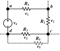
The sum of all the voltages around the loop is equal to zero. v1 + v2 + v3 + v4 = 0
This law is also called Kirchhoff's second law, Kirchhoff's loop (or mesh) rule, and Kirchhoff's second rule.
The principle of conservation of energy implies that the directed sum of the electrical potential differences (voltage) around any closed circuit must be zero.
Multimeters
Before using multimeters, one must identify what quantity is to be measured and also we need preparations of the dials, measuring cables, and familiarization with its functions. First thing you need to do is to check if your multimeter is in a good condition, check battery, output screens needs to be functional to read the obtained values to do some measurements. After that an operating procedure needs to be followed:
1. Set dial for the mode of measurement: AC/DC voltage, AC/DC current, AC/DC resistance.
2. Set the proper range. For the Voltage and Current measurements, always use maximum range.
3. Connect measuring cables to their proper terminals. Red for positive terminals and Black for negative terminals. The negative is usually denoted as ground (GND) or COMMON.
4. Zero adjustment setting for Ohmmeters. Adjust needle to zero adjustment by shorting.
5. Ready for measuring voltage, current and resistance.
Voltage Measurements
Voltages can be measured across any points in the circuit. These points refer to the positive terminal and the negative terminal of where the resistor is connected. When current is flowing through the circuit, there exist the potential differences from different points of the circuit. A correct correspondence of the readings depends on the proper connection of the measuring cables and should always be connected from the positive terminal to the negative terminal. The range of the voltmeter should be set to maximum range because we need the correct number of significant figures the meter can give and is used to obtain the voltage across to any points in the circuit. An infinitely large reading of internal resistance can be obtained if the instrument is ideal.
Current Measurements
Current can be measured from a part of a circuit. Such parts include the resistor and the capacitor. An ammeter is inserted in between the two points. Thus wire is disconnected from a connection. This allows the current to absorb the flow passing through the component of the circuit then goes through the ammeter. If an ideal ammeter is used, then a zero internal resistance can be obtained. The measuring cables must be inserted in the proper terminals because if it is inserted across the power source, the measuring needle for the AMM will break because it is very thin. Remember to always use a maximum range setting for proper readings of values.
Resistance Measurements
Resistance is measured by an ohmmeter. Resistors also have color codes which you can obtain the resistance of the resistors by means of nominal values. Resistors from the circuit contain the resistance that we need to measure. Since the resistance of an element is in passive quantity, thus before measuring the resistance of the element, we need to get first the current. No power source is needed in measuring the resistance that is why the internal circuitry contains a battery. Appropriate scales are set in order to obtain the values. The terminals also need to be shorted because of insufficiency of voltage from the battery. This is done by the tips of the measuring cables must touch with each other. Interference can also occur in the set-up so better check if it is properly in place.
Differentiate Digital Multimeter from an Analog Multimeter.
Digital and analog multimeters have many differences in common. The digital MM is more expensive than the analog MM and is much easier to use. The Analog MM displays the measure value by a needle and moves along a scale while a digital MM displays the result directly using 3 or more digits from its screen. The digital MM uses internal power source which is provided by a dry cell. Both multimeters differ in readings because of certain deflections. Although they have many comparisons with each other, the both of them can obtain measured values using different settings from a circuit.
How is Kirchhoff’s rules applied?
A branch point in a network is a point where three or more conductors are joined. A loop is any closed conducting path. Kirchhoff’s rules consist of two following statements: the point rule and the loop rule.
Point rule or junction rule states that the algebraic sum of the currents toward any branch is zero.
The current entering any junction is equal to the current leaving that junction. i1 + i4 = i2 + i3
This law is also called Kirchhoff's point rule, Kirchhoff's junction rule (or nodal rule), and Kirchhoff's first rule.
The principle of conservation of electric charge implies that:
At any node (junction) in an electrical
circuit,
the sum of currents flowing into that node is equal
to the sum of currents flowing out of that node.
The second statement which is the
Loop rule states that the algebraic sum of the potential differences in any
loop including those associated with EMFs and those of resistive elements must
equal to zero.
The sum of all the voltages around the loop is equal to zero. v1 + v2 + v3 + v4 = 0
This law is also called Kirchhoff's second law, Kirchhoff's loop (or mesh) rule, and Kirchhoff's second rule.
The principle of conservation of energy implies that the directed sum of the electrical potential differences (voltage) around any closed circuit must be zero.
This was one of my projects constructed during my college years. It is a digital chess game clock which can be operated at 9:00 minutes blitz game with 2 players competing in a game of chess. Time is accommodated for each player for each move they make. Several buttons and switches are used for setting the time, start and stop, and for reset. Each player touches a switch to stop his time and starts the opponent’s time. The game will end when the time will expire and it will determine the winner of the chess game.
The Plan:
My designs were based on a standard chess game clock except for the time setting. I chose a time setting which is intended for amateurs in chess games. My design were composed of two timers with set buttons for seconds and switch button for players. A 1 Hz clock pulse oscillator is also implemented in the timer for countdown purposes.
SWITCH and RESET BUTTONS
The set buttons are connected to pin 14 (CLK) and then to the 74LS08 on their pin 3. Pins 1 and 2 of the same IC then is connected to pin 7 (Q3) of 74LS190 which is the flip flop output.
The on/off switch which is a single pole – dual throw switch is connected to pin 14 (CLK) of the 74LS190 on the upper side circuit.
The dual pole – dual throw switch is connected to the on/off switch. The upper pole of the dual pole – dual throw switch is connected to the 1 Hz oscillator. The lower pole is connected to the 1 Hz oscillator and to pin 14 (CLK) of the lower side circuit.
2N222 transistors are also implemented so that the count for the set buttons will be descending to 0. The 2N222 transistor is connected to pin 11 (PL) Parallel load control input, and the base and emitter is connected to pin 7(Q3) and GND.
DISPLAY
The display used in the design is a common cathode BCD 7-segment decoder. I only used 3 digits for the dual timer. 470K resistors were connected to each pin of the decoder so that it will prevent overdrive of the LEDs. The 7 segment decoder is then connected to 74LS48 IC to their pins 9 to 14 which are the outputs for the display. The BCDA inputs which are the pins 1, 2, 6 and 7 are then connected to the flip flop outputs from the 74LS190 pins 3, 2, 6 and 7. The first IC of 74LS190 the parallel inputs pin 15, 1, 10 and 9 identified. Pins 1 and 9 were connected to Vcc=5V and pins 15 and 10 were connected to ground. The display in in the 7 segment decoder will now be on number 9. Next the second IC of 74LS190 parallel inputs were connected to display a certain number 5. Pins 15 and 10 were connected to Vcc=5V and pins 1 and 9 were connected to ground. The reading then displays the number 5.
THE OSCILLATOR

Explain here
A crystal oscillator is an electronic circuit that uses the mechanical resonance of a vibrating crystal of piezoelectric material to create an electrical signal with a very precise frequency. This frequency is commonly used to keep track of time (as in quartz wristwatches), to provide a stable clock signal for digital integrated circuits, and to stabilize frequencies for radio transmitters. The crystal oscillator circuit sustains oscillation by taking a voltage signal from the quartz resonator, amplifying it, and feeding it back to the resonator. The rate of expansion and contraction of the quartz is the resonant frequency, and is determined by the cut and size of the crystal.
A crystal oscillator is an electronic circuit that uses the mechanical resonance of a vibrating crystal of piezoelectric material to create an electrical signal with a very precise frequency. This frequency is commonly used to keep track of time (as in quartz wristwatches), to provide a stable clock signal for digital integrated circuits, and to stabilize frequencies for radio transmitters. The crystal oscillator circuit sustains oscillation by taking a voltage signal from the quartz resonator, amplifying it, and feeding it back to the resonator. The rate of expansion and contraction of the quartz is the resonant frequency, and is determined by the cut and size of the crystal.
Resonance modes
A quartz crystal provides both series and parallel resonance. The series resonance is a few kilohertz lower than the parallel one. Crystals below 30 MHz are generally operated between series and parallel resonance, which means that the crystal appears as an inductive reactance in operation. Any additional circuit capacitance will thus pull the frequency down. For a parallel resonance crystal to operate at its specified frequency, the electronic circuit has to provide a total parallel capacitance as specified by the crystal manufacturer.
Crystals above 30 MHz (up to >200 MHz) are generally operated at series resonance where the impedance appears at its minimum and equal to the series resistance. For these crystals the series resistance is specified (<100 Ω) instead of the parallel capacitance. To reach higher frequencies, a crystal can be made to vibrate at one of its overtone modes, which occur near multiples of the fundamental resonant frequency. Only odd numbered overtones are used. Such a crystal is referred to as a 3rd, 5th, or even 7th overtone crystal. To accomplish this, the oscillator circuit usually includes additional LC circuits to select the desired overtone.
Circuit's Upper Portion:

Circuit's Lower Portion:

The Final Circuit

Magnetic Levitator is a closed loop system that lets an object suspend without any assistance but with the support of magnetic fields. The said magnetic field comes from the wounded coil.
The Process
A ferromagnetic ball is to be kept suspended on the air through the use of an electromagnet without any contact in between them. Hence, the process is called magnetic levitation. A distance from the core head of the electromagnet to the center if the ball is set. This becomes the reference distance. When the ball goes beyond or below the reference distance, the magnetic force of attraction of the electromagnet will vary accordingly to compensate for the change in location of the ball. Thus, the ball is kept levitated. This Magnetic Levitator uses a light sensor that will control the voltage in order to make the ball levitate. This project involves the principles of electromagnetism and also involves control system design of a closed loop system that means it must be a self-correcting device that will auto correct if there will be and error that has been returned to the system.
SYSTEM MODEL
a) Theoretical Modeling
The Magnetic Levitator Modeling:


The magnetic levitator’s physical structure includes the following subsystems:
- Electromagnet mounted in a rectangular frame
- Power supply with different DC voltage outputs
- Sensors: using LED (Light Emitting Diode) and LDR (Light Dependent Resistor) used as positioned at the stand
- PD (Proportional-Derivative) Controller set-up on the breadboard which composes the following:
· Op-Amp (LM741)
· Power transistor (2N3055)
· Resistors
· Potentiometers
· Capacitors
· Connecting Wires

c) Parameter Determination
The different parameters were required in order to construct a successful controller. The following values were obtained from the measurements done.
M= 0.020 kg
g= 9.81 m/s2
io=0.8 A
yo=0.015 m
L= 0.022401 H
R= 8.869 ohms
d) Final Plant Model
Substituting the gathered parameters to the state-space model equation:


THE CONTROLLER
a) Design
An effective controller must be able to control and hold the position of the ferromagnetic ball for a certain period of time. The controller manipulates the magnetic field intensity across the coil by tuning the appropriate voltage across the coil so as to keep the ball suspended in stability.
From the final plant model, we have obtained the matrices, transfer function and the sensor model. Using the Matlab SisoTool, we obtained the values of C(s).


The Process
A ferromagnetic ball is to be kept suspended on the air through the use of an electromagnet without any contact in between them. Hence, the process is called magnetic levitation. A distance from the core head of the electromagnet to the center if the ball is set. This becomes the reference distance. When the ball goes beyond or below the reference distance, the magnetic force of attraction of the electromagnet will vary accordingly to compensate for the change in location of the ball. Thus, the ball is kept levitated. This Magnetic Levitator uses a light sensor that will control the voltage in order to make the ball levitate. This project involves the principles of electromagnetism and also involves control system design of a closed loop system that means it must be a self-correcting device that will auto correct if there will be and error that has been returned to the system.
SYSTEM MODEL
a) Theoretical Modeling
The Magnetic Levitator Modeling:
Figure 1. Theoretical Block Diagram
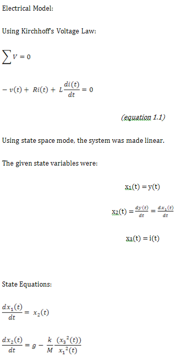
Figure 2. Magnetic Levitator Model
Mechanical Model:
Newton’s Law of Equilibrium:
Newton’s Law of Equilibrium:
b. Plant Contstruction
Physical Construction Design
Figure 3. Physical Design
The magnetic levitator’s physical structure includes the following subsystems:
- Electromagnet mounted in a rectangular frame
- Power supply with different DC voltage outputs
- Sensors: using LED (Light Emitting Diode) and LDR (Light Dependent Resistor) used as positioned at the stand
- PD (Proportional-Derivative) Controller set-up on the breadboard which composes the following:
· Op-Amp (LM741)
· Power transistor (2N3055)
· Resistors
· Potentiometers
· Capacitors
· Connecting Wires
Power Supply Rating:
Voltage
|
Function
|
+5V
|
Light Source Supply (LED)
|
+12V
|
Sensor Supply (LDR), Coil & Power Transistor Supply
|
+12V/-12V
|
Controller Op-Amp Supply
|
c) Parameter Determination
The different parameters were required in order to construct a successful controller. The following values were obtained from the measurements done.
M= 0.020 kg
g= 9.81 m/s2
io=0.8 A
yo=0.015 m
L= 0.022401 H
R= 8.869 ohms
d) Final Plant Model
Substituting the gathered parameters to the state-space model equation:
G(s) =C*inv(s*I-A)
We obtained the following matrices:
The final plant transfer function is:
The sensor model can be represented by its characteristics slope. This was done by observing the voltage across the sensor with respect to the changes in ball position.
The sensor model was,
H(s) = -503
THE CONTROLLER
a) Design
An effective controller must be able to control and hold the position of the ferromagnetic ball for a certain period of time. The controller manipulates the magnetic field intensity across the coil by tuning the appropriate voltage across the coil so as to keep the ball suspended in stability.
From the final plant model, we have obtained the matrices, transfer function and the sensor model. Using the Matlab SisoTool, we obtained the values of C(s).
The compensator equation was, C(s) = 6.19(1 0.013s)
The figure above shows the block diagram representation of the control feedback
analysis of the magnetic levitation system.
b. Implementation
A PD controller was in used in the magnetic levitator system:
Circuit Diagram:
Using Matlab root locus plot, the values C1, R1, R2, R3, and R4 were obtained by equating to C(s):
C(s) = -R2C1(s+(1/(R2C1)))
C(s) = -619(1+0.018s)
6.19 = R2/R1
6.19 * 0.018 = C2R2
if C2 = 4,7uF
R2 = 50.6K ohms
R1 = 8K ohms
RESULTS
(on the left): ferrite ball; (right) magnetic levitator set-up
Schematic Diagram

Materials Used

Materials Used
System Performance
The results of the project show that the voltage across the controller and its components change as the ball blocks shadows the light entering the tube where the LDR is located. This shows that the controller is actuated when it senses the change in the sensor voltage. When the position of the ball changes, the sensor voltage sends a signal triggering the controller to increase or decrease its output voltage depending to what the system warrants. The controller output is then fed to a power transistor whose collector terminal is connected to the other end of the coil. The voltage variations across the coil control the intensity of the magnetic flux, ultimately controlling the magnetic force that acts on the ball. A potentiometer is connected in series with the power transistor’s base terminal in order to properly bias the device.
Problems Encountered and Troubleshooting
I'd encountered several problems working with the project design and implementation. The intricacy in obtaining a working controller delayed much of the progress. The controller op-amps were found to saturate resulting to a constant controller output. The controller eventually worked when the researchers changed the compensator values. Another problem was the difficulty in controlling the “pocket” under the electromagnet. By improving the bolt head, from edged to rounded, the pocket drastically improved.
CONTROL SYSTEM CONCEPTS LEARNED
Control systems influence each facet of modern life. The portion of the system to be controlled is called the plant or the process. It is affected by applied signals, called inputs, and produces signals of particular interest, called outputs. (Stefani, 1982).
When an open-loop control cannot compensate the requirements of a system, a closed-loop system is desirable. One of the most powerful tools of control-system analysis and design is the transfer function representation. Using the transfer function, a plant can be modeled into its graphical or mathematical representation. Proficiency in Laplace Transform is an advantage in the analysis of transfer functions. The translation from time to frequency domain made the response analysis easier.
From Root Locus analysis we learned that when even one pole is at the right half of the plain, the system is said to be unstable. By introducing compensators, the root locus plot can be greatly controlled. This is done by adding zeros or poles to the system
Aside from classical control, the modern control was also introduced in the design and theoretical modeling of the system. Using State-space analysis, the matrix components of the model was derived. State space refers to the space whose axes are the state variables. The state of the system can be represented as a vector within that space. State-space analysis is a more advanced approach of control engineering.
CONCLUSION
The ferromagnetic ball levitates because of the controller’s function. The process begins with the sensor sending signal to the controller which is then converted into magnetic force acting on the ball. The latter is varied depending on what the system requires. In general, the controller compensates the system’s inadequacy in obtaining the desired output. The system’s stability is directly affected by its parameters, plant model and controller design and ambient environment as well. Therefore a good controller must be versatile enough to compensate with these changes.
Control system is very important in different fields of engineering especially in electrical and electronics since the world today demands a more automated and accurate system. Since control system is an interdisciplinary field of study it is highly encouraged that it be studied so that it will farther be developed.