Magnetic Levitator
Magnetic Levitator is a closed loop system that lets an object suspend without any assistance but with the support of magnetic fields. The said magnetic field comes from the wounded coil.
The Process
A ferromagnetic ball is to be kept suspended on the air through the use of an electromagnet without any contact in between them. Hence, the process is called magnetic levitation. A distance from the core head of the electromagnet to the center if the ball is set. This becomes the reference distance. When the ball goes beyond or below the reference distance, the magnetic force of attraction of the electromagnet will vary accordingly to compensate for the change in location of the ball. Thus, the ball is kept levitated. This Magnetic Levitator uses a light sensor that will control the voltage in order to make the ball levitate. This project involves the principles of electromagnetism and also involves control system design of a closed loop system that means it must be a self-correcting device that will auto correct if there will be and error that has been returned to the system.
SYSTEM MODEL
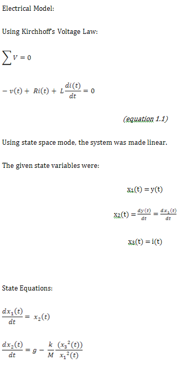
a) Theoretical Modeling
The Magnetic Levitator Modeling:


Newton’s Law of Equilibrium:


The magnetic levitator’s physical structure includes the following subsystems:
- Electromagnet mounted in a rectangular frame
- Power supply with different DC voltage outputs
- Sensors: using LED (Light Emitting Diode) and LDR (Light Dependent Resistor) used as positioned at the stand
- PD (Proportional-Derivative) Controller set-up on the breadboard which composes the following:
· Op-Amp (LM741)
· Power transistor (2N3055)
· Resistors
· Potentiometers
· Capacitors
· Connecting Wires
Voltage
|
Function
|
+5V
|
Light Source Supply (LED)
|
+12V
|
Sensor Supply (LDR), Coil & Power Transistor Supply
|
+12V/-12V
|
Controller Op-Amp Supply
|

c) Parameter Determination
The different parameters were required in order to construct a successful controller. The following values were obtained from the measurements done.
M= 0.020 kg
g= 9.81 m/s2
io=0.8 A
yo=0.015 m
L= 0.022401 H
R= 8.869 ohms
d) Final Plant Model
Substituting the gathered parameters to the state-space model equation:


THE CONTROLLER
a) Design
An effective controller must be able to control and hold the position of the ferromagnetic ball for a certain period of time. The controller manipulates the magnetic field intensity across the coil by tuning the appropriate voltage across the coil so as to keep the ball suspended in stability.
From the final plant model, we have obtained the matrices, transfer function and the sensor model. Using the Matlab SisoTool, we obtained the values of C(s).


Materials Used

The results of the project show that the voltage across the controller and its components change as the ball blocks shadows the light entering the tube where the LDR is located. This shows that the controller is actuated when it senses the change in the sensor voltage. When the position of the ball changes, the sensor voltage sends a signal triggering the controller to increase or decrease its output voltage depending to what the system warrants. The controller output is then fed to a power transistor whose collector terminal is connected to the other end of the coil. The voltage variations across the coil control the intensity of the magnetic flux, ultimately controlling the magnetic force that acts on the ball. A potentiometer is connected in series with the power transistor’s base terminal in order to properly bias the device.
Problems Encountered and Troubleshooting
I'd encountered several problems working with the project design and implementation. The intricacy in obtaining a working controller delayed much of the progress. The controller op-amps were found to saturate resulting to a constant controller output. The controller eventually worked when the researchers changed the compensator values. Another problem was the difficulty in controlling the “pocket” under the electromagnet. By improving the bolt head, from edged to rounded, the pocket drastically improved.
CONTROL SYSTEM CONCEPTS LEARNED
Control systems influence each facet of modern life. The portion of the system to be controlled is called the plant or the process. It is affected by applied signals, called inputs, and produces signals of particular interest, called outputs. (Stefani, 1982).
When an open-loop control cannot compensate the requirements of a system, a closed-loop system is desirable. One of the most powerful tools of control-system analysis and design is the transfer function representation. Using the transfer function, a plant can be modeled into its graphical or mathematical representation. Proficiency in Laplace Transform is an advantage in the analysis of transfer functions. The translation from time to frequency domain made the response analysis easier.
From Root Locus analysis we learned that when even one pole is at the right half of the plain, the system is said to be unstable. By introducing compensators, the root locus plot can be greatly controlled. This is done by adding zeros or poles to the system
Aside from classical control, the modern control was also introduced in the design and theoretical modeling of the system. Using State-space analysis, the matrix components of the model was derived. State space refers to the space whose axes are the state variables. The state of the system can be represented as a vector within that space. State-space analysis is a more advanced approach of control engineering.
CONCLUSION
The ferromagnetic ball levitates because of the controller’s function. The process begins with the sensor sending signal to the controller which is then converted into magnetic force acting on the ball. The latter is varied depending on what the system requires. In general, the controller compensates the system’s inadequacy in obtaining the desired output. The system’s stability is directly affected by its parameters, plant model and controller design and ambient environment as well. Therefore a good controller must be versatile enough to compensate with these changes.
Control system is very important in different fields of engineering especially in electrical and electronics since the world today demands a more automated and accurate system. Since control system is an interdisciplinary field of study it is highly encouraged that it be studied so that it will farther be developed.
k=?
ReplyDelete